Sorting
Table of Contents
1. Sorting
Sorting solves the problem of putting a set of elements in order. To put a set of elements in order, there must be some relation \(<\) that we can define for those elements that satisfy two conditions:
- Law of Trichotomy: Exactly one of \(a < b\), \(a = b\), or \(b < a\) is true.
- Law of Transitivity: If \(a < b\) and \(b < c\), then \(a < c\).
An inversion is a pair of elements that are out of order with respect to our relation \(<\).
2. Comparison Sorts
2.1. Selection Sort
To selection sort \(N\) items, we:
- Find the smallest item in the unsorted portion of the array.
- Swap it to the end of the sorted portion of the array.
- Selection sort the remaining unsorted items.
The time complexity of selection sort is \(N + (N-1) + \cdots + 1 = \Theta(N^2)\), and the space complexity is \(\Theta(1)\) because we do not need extra memory.
2.2. Heap Sort
Selection sort is inefficient because we have to search the entire unsorted array for the smallest item every time. The fix is to first insert all the items into a max heap.
To heap sort \(N\) items, we can then:
- Delete largest item from the max heap.
- Put deleted item at the first open slot starting from the end of our output array.
The time complexity of heap sort is \(O(N \log N)\). The space complexity of heap sort is the memory we need to build the copy of our data, so it is \(\Theta (N)\).
2.2.1. In-Place Heap Sort
To increase memory efficiency, instead of using a separate output array, we can use the same input array and sort in-place. First, we can create a complete binary tree directly using the elements in our input array, and then “heapify” the result. To do this, we:
- Sink nodes in reverse level order.
- After sinking, we guarantee that the tree rooted at that node is a heap.
Now that we have our heap, we can run heap sort in-place like so:
- Delete largest item from the max heap by swapping the root with the last item in the heap.
- Sink until the heap is valid again.
- Repeat for all \(N\) items.
Then, the resulting array is sorted:
Now, our space complexity is just \(\Theta(1)\) since we don’t need any extra memory.
2.3. Merge Sort
To merge sort \(N\) items, we:
- Split items into two roughly even pieces.
- Merge sort each half recursively.
- Merge the two sorted halves to form the final result
To merge two sorted halves together, we compare elements from the first half with elements from the second half, and build a new auxiliary array:
The time complexity for this is \(\Theta(N \log N)\), and its space complexity is \(O(N)\).
2.4. Insertion Sort
To insertion sort \(N\) items, we:
- Start with an empty output sequence.
- Add each item from the input, inserting into the output at the right point.
We can also do this in-place by maintaining a sorted and unexamined section of the input array. To insert, we can swap item backwards until it is in the right place among all previously sorted items:
The best case time complexity is \(\Theta(N)\) (when it is already sorted), and the worst case time complexity is \(\Theta(N^2)\). Realize that when an array that is almost sorted, insertion sort does very little work due to its best case time complexity. Additionally, for small arrays (\(N < 15\) or so), insertion sort is fastest.
2.5. Quicksort
The idea behind quicksort is that for an array, we can pick one item (called the pivot), get it in the correct spot, and then just ensure that the rest of the items are on the correct side:
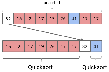
If we then run quicksort recursively on the two subarrays on the left and right of the pivot, we end up with a sorted array. The process of picking the pivot to split the array up into left and right subarrays is called partitioning.
2.5.1. Naive Partitioning
Naively, we can simply create another array. Then, we can scan through the array, adding the elements smaller than our pivot at the front. Then, we add our pivot. Finally, we scan through the array again, adding all the elements greater than our pivot at the back.
2.5.2. Hoare Partitioning
A faster way is to have two pointers walk towards each other. The left pointer favors items smaller than the pivot, whereas the right pointer favors items larger than the pivot. The idea is that they walk towards each other, swapping anything they don’t like.
More specifically, both pointers step towards each other. Each pointer stops when they find an element they don’t like. When both pointers stop, they swap their elements with each other, and then move on. When both pointers cross, all that is left to do is to swap the pivot to the right spot:
2.5.3. Runtime
The runtime for quicksort highly depends on what element you choose as the pivot. It turns out that it is fastest if we choose the median as the pivot. With this in mind, the best case time complexity for quicksort is \(\Theta(N \log N)\), and worst case it is \(\Theta(N^2)\).
But how is it better than mergesort if the worst case it is \(\Theta(N^2)\)? It turns out that with analysis, the average runtime of quicksort is \(\Theta(N \log N)\), and it is faster than mergesort.
Usually, however, most pivots we choose come out to a runtime of \(\Theta(N \log N)\). What we need to do is to figure out how to avoid the worst case. The worst case happens when the array is already in sorted order (or almost sorted order). To avoid this, we can employ a few different strategies:
- Randomness: pick a random pivot or shuffle before sorting.
- Smarter pivot selection: calculate or approximate the median
- Introspection: switch to a safer sort if recursion goes too deep
- Preprocess: analyze first to see if quicksort would be slow (no obvious way to do this)
3. Theoretical Bound on Comparison Sorts
Of the comparison sorts above, the best time complexity is \(O(N\log N)\). We also know that for a comparison sorting algorithm, we must at least look at every element in the array (\(\Omega(N)\)). The question is, is there a better lower bound we can find, i.e. an algorithm that can theoretically run faster than \(\Theta(N\log N)\) in the worst case?
It turns out that the best possible worst-case time complexity of a sorting algorithm using comparisons is \(\Theta(N \log N)\). This is because if you look at the decision tree of sorting \(N\) items, you must make \(\log N!\) comparisons to definitively know the items are sorted. Then, it can be shown that \(\log N! \in \Omega(N \log N)\), so the best time complexity we can find is \(\Theta(N \log N)\).
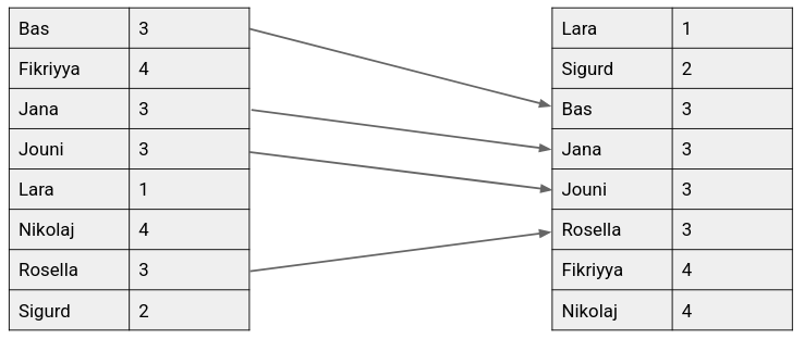
4. Sorting Stability
A sort is said to be stable if the order of equivalent items is preserved:
5. Non-Comparison Sorts
Since comparison sorts are limited to \(\Theta(N\log N)\) time complexity, perhaps we can achieve better time complexity for sorting certain special sets.
5.1. Counting Sort
Counting sort exploits the space instead of time. Say we have a list of names that have IDs ranging from 0 to 11. Then, we can sort this list of names by ID by simply relating their ID to an index in an array.
Running this algorithm, we would be able to sort \(N\) items in \(\Theta(N)\) worst case time.
More generally, we call the set of possible indices that our keys can take on the alphabet. Then, if our alphabet is of size \(R\) and we have \(N\) keys, counting sort runs in \(\Theta(N+R)\) worst case time.
5.2. Radix Sort
Counting sort is slow when our alphabet is large. By decomposing our input keys into a string of characters from a finite alphabet, we can force \(R\) ot be small. We can sort each digit independently from the rightmost digit (least significant digit) towards the left by running counting sort independently on each digit, or radix.
Then, the runtime of this algorith mis \(\Theta(WN+WR)\), where \(N\) is the number of items, \(R\) is the size of the alphabet, and \(W\) is the width of each item in digits.