Probability

An event \(B \subseteq \Omega\) is said to be partitioned into \(n\) events \(B_1, \dots , B_n\) if the following conditions are satisfied:

1. \(B = B_1 \cup B_2 \cup \cdots \cup B_n\)
2. \(B_i \cap B_j = \varnothing \; \forall i \neq j\) (that is, \(B_1, \dots, B_n\) are mutually exclusive)

Then, the following properties are satisfied for any valid probability space:

• Non-negativity: \(\mathbb{P}(A) \geq 0 \; \forall A \subseteq \Omega\)
• Countable Additivity: if \(B_1, B_2, \dots, B_n\) are partitions of \(B\), then

\begin{align} \mathbb{P}(B) = \sum_{k=1}^n \mathbb{P}(B_k), \quad \forall B \subseteq \Omega \notag \end{align}

• Normalization: \(\mathbb{P}(\Omega) = 1\)

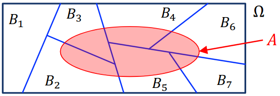
Suppose \(B_1, \dots, B_n\) are partitions of \(\Omega\). Then, for any \(A \subseteq \Omega\), we have:

\begin{align} \boxed{\mathbb{P}(A) = \sum_{i=1}^n \mathbb{P}(A | B)\mathbb{P}(B_i)} \end{align}

This is true because we see that it becomes the sum of the intersections of each partition \(B_i\) with \(A\):

Suppose \(B_1, \dots, B_n\) partition \(\Omega\). Then, for any \(A \subseteq \Omega\), with \(\mathbb{P}(A) > 0\), we have:

\begin{align} \mathbb{P}(B_i | A) = \frac{\mathbb{P}(A | B_i)\mathbb{P}(B_i)}{\mathbb{P}(A)} = \frac{\mathbb{P}(A|B_i)\mathbb{P}(B_i)}{\sum_{j=1}^n \mathbb{P}(A|B_j)\mathbb{P}(B_j)} \end{align}

Intuitively, if \(A\) is some event we are studying, then the \(B_i\) partitions are the different “ways” that event can occur (e.g. a positive test result is \(A\), then real positive and false positive are two ways that can occur). Bayes’ rule tells us that the probability it is one of those ways is equal to the probability of \(A \cap B_i\) happening (\(A\) happening via \(B_i\)) over the total probability of \(A\) happening.

Consider any two events \(A, B \subseteq \Omega\) and suppose that the chance of \(A\) does not depend on whether or not \(B\) occurs, i.e. \(\mathbb{P}(A | B) = \mathbb{P}(A | B^C)\). Then, since \(B\) and \(B^C\) partitions \(\Omega\), by the Law of Total Probability:

\begin{align} \mathbb{P}(A) &= \mathbb{P}(A | B)\mathbb{P}(B) + \mathbb{P}(A|B^C)\mathbb{P}(B^C) \notag \\ &= \mathbb{P}(A|B)\left(\mathbb{P}(B)+\mathbb{P}(B^C)\right) \notag \\ &= \mathbb{P}(A|B) \notag \end{align}

Then, if \(A\) and \(B\) are independent, by (3) we know that \(\mathbb{P}(A \cap B) = \mathbb{P}(A | B)\mathbb{P}(B)\). But \(\mathbb{P}(A | B) = \mathbb{P}(A)\), so:

\begin{align} \boxed{\mathbb{P}(A\cap B) = \mathbb{P}(A)\mathbb{P}(B)} \end{align}

Considering the box model, this means that in our probability space, the events of \(A\) and \(B\) must overlap in a very specific way such that either \(A\) or \(B\) happening tells us nothing about the other. To achieve this, the proportion of \(B\) that falls inside \(A\) must be exactly the same as the proportion of \(B\) with respect to the entire box.

This implies that the complements of the events must also be independent:

• \(\mathbb{P}(A^C \cap B) = \mathbb{P}(A^C)\mathbb{P}(B)\)
• \(\mathbb{P}(A \cap B^C) = \mathbb{P}(A)\mathbb{P}(B^C)\)
• \(\mathbb{P}(A^C \cap B^C) = \mathbb{P}(A^C)\mathbb{P}(B^C)\)

For events \(A_1,\dots,A_n\) on the same probability space, the product rule says that:

\begin{align} \boxed{\mathbb{P}(A_1 \cap \cdots \cap A_n) = \mathbb{P}(A_1)\mathbb{P}(A_2|A_1)\mathbb{P}(A_3|A_1\cap A_2) \cdots \mathbb{P}(A_n|A_1 \cap \cdots \cap A_{n-1})} \end{align}

Intuitively, this just says that the probability of events \(A_1\) through \(A_n\) happening is just the probability of \(A_1\) happening, times the probability of \(A_2\) happening after \(A_1\) has happened, and so on.

Proof: We proceed by induction on \(n\). The base case of \(n=1\) holds since \(\mathbb{P}(A_1) = \mathbb{P}(A_1)\).

Assume that the product rule holds for all \(n \leq k\). Then, for \(n=k+1\), we have:

\begin{align} \mathbb{P}(A_1 \cap \cdots \cap A_{k+1}) = \mathbb{P}\left(\left(\bigcap_{i=1}^k A_i\right) \cap A_{k+1}\right) \notag \end{align}

Let’s call the event \(B=\bigcap_{i=1}^k A_i\). Then, we have:

\begin{align} \mathbb{P}(A_1 \cap \cdots \cap A_{k+1}) &= \mathbb{P}(B \cap A_{k+1}) \notag \\ &= \mathbb{P}(B)\mathbb{P}(A_{k+1}|B) \notag \end{align}

By the inductive hypothesis, \(\mathbb{P}(B) = \mathbb{P}(A_1)\cdots\mathbb{P}(A_k|A_1\cap \cdots \cap A_{k-1})\), so we find that our expression is equal to \(\mathbb{P}(A_1) \cdots \mathbb{P}(A_{k+1}|A_1 \cap \cdots \cap A_k)\), and we are done. \(\square\)

Hashing uses a hash function \(h: U \rightarrow T\) to map an input from a large domain into a fixed-size representation, where \(U\) is the universe of keys and \(T\) is the space of our hash table.

We can model a hash function as mapping each key uniformly at random to \(n\) labelled bins. However, we want to minimize the probability that a collision will occur (i.e. two keys maps to the same location). The question is, for a given hash table size \(n\) and some \(\epsilon > 0\), what is the largest number of keys \(m\) such that the probability of collision is less than \(\epsilon\)?

The number of pairs of keys is \(\binom{m}{2}\). For \(i\) in \(1, ..., \binom{m}{2}\), let \(C_i\) be the event that pair \(i\) collides. Then, the probability \(\mathbb{P}(C_i) = \frac{1}{n}\), as there is one slot out of the \(n\) locations that the second key can pick to collide with the first.

Then the probability of the event \(C\) that at least one pair collides is given by the union \(\bigcup_{i=1}^{\binom{m}{2}}C_i\). Then, by union bound, we have:

\begin{align} \mathbb{P}\left(\bigcup_{i=1}^{\binom{m}{2}}C_i\right) & \leq \sum_{i=1}^{\binom{m}{2}}\mathbb{P}(C_i) \notag \\ &= \binom{m}{2}\frac{1}{n} \notag \\ &\leq \frac{m^2}{2}\frac{1}{n} \notag \end{align}

Thus, we want to find \(m\) such that \(frac{m^2}{2}\frac{1}{n} \leq \epsilon\). This is satisfied when:

\begin{align} m \leq \sqrt{2\epsilon n} \notag \end{align}

Say we have \(m\) identical jobs that we wish to load balance across \(n\) identical processors. Define \(L_i\) as the load (i.e. number of jobs) of processor \(i\). Call event \(A_k\) to be the event that some processor has a load of at least \(k\). Then, the event \(\bar{A}_k\) is the event that all processors have less than \(k\) jobs. We want to find the smallest \(k\) such that \(\mathbb{P}(\bar{A}_k) \geq \frac{1}{2}\) (i.e. the smallest \(k\) such that the probability that all processors have less than \(k\) jobs allocated to them is greater than half). Equivalently, we want to find \(k\) such that \(\mathbb{P}(A_k)\leq\frac{1}{2}\).

We know that \(\mathbb{P}(A_k) = \mathbb{P}\left(\bigcup_{i=1}^{n} \left(L_i \geq k\right)\right)\). Then, by union bound:

\begin{align} \mathbb{P}\left(\bigcup_{i=1}^{n} \left(L_i \geq k\right)\right) &\leq \sum_{i=1}^n\mathbb{P}(L_i \geq k) \notag \\ &= n \mathbb{P}(L_1 \geq k) \notag \end{align}

Say \(B_S\) is the event that all jobs in some subset \(S \subseteq \{1, \dots, m\}\) land in bin 1 (i.e. processor 1). Since each job has probability \(\frac{1}{n}\) in landing in processor 1, the probability of \(B_S\) is \(\mathbb{P}(B_S) = \frac{1}{n^{|S|}}\).

Then, the event \(L_1 \geq k\) is just the union of events \(B_S\) such that \(S\) is all the possible subsets of the jobs such that \(S\) is of size \(k\). Thus, by union bound:

\begin{align} \mathbb{P}(L_1 \geq k) &\leq \sum_{S \subseteq \{1, \dots, m\}: |S|=k} \mathbb{P}(B_S) \notag \\ &= \binom{m}{k} \frac{1}{n^k} \notag \end{align}

Say \(n=m\) (number of processors is equal to number of jobs). Then, \(\mathbb{P}(A_k) \leq n\binom{n}{k}\frac{1}{n^k} \leq \frac{n}{k!}\). Thus, \(k\) just needs to satisfy \(\frac{n}{k!} \leq \frac{1}{2}\).

Say we have \(n\) distinct coupons, with \(1\) coupon per box. All coupon types are equally likely to be in any give box, and we wish to collect all \(n\) distinct coupons to “win.” Let \(A_i\) be the event that coupon \(i\) is not collected after \(m\) purchases.

We can think of this problem as throwing \(m\) unlabelled balls uniformly at random into \(n\) labelled bins. The probability that some coupon is not collected is:

\begin{align} \mathbb{P}\left(\bigcup_{i=1}^n A_i\right) &\leq \sum_{i=1}^n\mathbb{P}(A_i) \notag \\ &= n\mathbb{P}(A_1) \notag \\ &= n\left(1-\frac{1}{n}\right)^m \notag \end{align}

Since \(\left(1-\frac{1}{n}\right)^n \approx e^{-1}\) as \(n\) approaches infinity, we can write the probability approximately as \(ne^{-\frac{m}{n}}\). Suppose we want \(\mathbb{P}\left(\bigcup_{i=1}^n A_i\right) \leq e^{-1} \approx 0.368\). Then, solving for \(m\), we find that \(m \geq n\ln n + n\).