Complex Exponentials
Table of Contents
1. Complex Exponentials
Consider the following complex exponential with the following properties:
\begin{align} x: \mathbb{R} &\rightarrow \mathbb{C} \notag \\ x(t) &= e^{it} \notag \\ x(0) &= 1 \notag \\ \dot{x}(t) &= ie^{it} \notag \end{align}We claim this is actually just the unit circle in the complex plane. Consider the function as a "particle," with its time derivative (velocity) plotted below:
But, this is just circular motion! Additionally, since the speed of the particle is just the magnitude of the velocity, we have:
\begin{align} |\dot{x}(t)| = |ie^{it}| = 1 \notag \end{align}More generally, a complex exponential of the following form moves at \(\omega\) radians per second:
\begin{align} \boxed{x(t) = e^{i\omega t}} \end{align}1.1. Euler's Formula
With this knowledge, we can represent the position of the particle at time \(t\) like so:
Since the speed of the particle is \(1\), at time \(t\) the particle would have moved \(t\) radians away from the center. With trigonometry, it is easy to see that we can represent this point as \(\cos t + i\sin t\). This yields the famous Euler's formula:
\begin{align} \boxed{e^{it} = \cos t + i \sin t} \end{align}Plugging \(-t\) into the formula,
\begin{align} e^{-it} = \cos t - i\sin t \notag \end{align}Adding and subtracting this with the original formula yields us the inverse Euler's formulas:
\begin{align} \boxed{\cos t = \frac{e^{it} + e^{-it}}{2}} \\ \boxed{\sin t = \frac{e^{it} - e^{-it}}{2i}} \end{align}2. DT Complex Exponentials
We can write discrete-time complex exponentials in the following way:
\begin{align} \boxed{x[n] = e^{i\omega n} = \cos(\omega n) + i\sin(\omega n) \quad \forall n \in \mathbb{Z}} \end{align}DT complex exponentials are \(2\pi\) periodic in \(\omega\), which means that \(e^{i(\omega + 2\pi)n} = e^{i\omega n}\). More generally, \(\omega\) determs the frequency at which the signal oscillates:
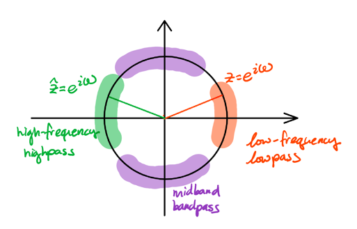
\begin{align} \omega &= 0 \Rightarrow x[n] = 1 \quad &\forall n \in \mathbb{Z} \notag \\ \omega &= \pi \Rightarrow x[n] = (-1)^n \quad &\forall n \in \mathbb{Z} \notag \end{align}When \(\omega = 0\), the signal oscillates the slowest (it is constant); on the other hand, \(\omega = \pi\) yields the fastest oscillating DT signal. We can categorize these frequencies as low-frequency, high-frequency, or midband: