Vectors and Signals

Continuous-time (CT) signals are signals \(x: \mathbb{R} \rightarrow \mathbb{R}\) or \(x: \mathbb{R} \rightarrow \mathbb{C}\) that take a continuous set as the domain. For example, \(\left[ \mathbb{R} \rightarrow \mathbb{R} \right]\) is the set of all real functions (signals) of a real variable, and \(\left[ \mathbb{R} \rightarrow \mathbb{C} \right]\) is the set of all complex signals of a real variable.

Discrete-time (DT) signals, on the other hand, are signals \(x: \mathbb{Z} \rightarrow \mathbb{R}\) or \(x: \mathbb{Z} \rightarrow \mathbb{C}\) that take a discrete set as the domain. We use \(x[n]\) to denote the value of a DT signal at a particular time (note the brackets, as opposed to parantheses for CT signals). We use a plot like the following for DT signals:

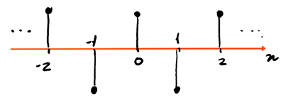
In this case, this is a plot of the function \(x[n] = \cos(\pi n)\).

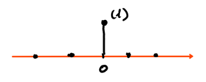
The Kronecker delta signal, also known as the discrete-time impulse, is a signal that is only 1 at zero:

\begin{align} \delta [n] = \begin{cases} 1 & n = 0 \\ 0 & n \neq 0 \\ \end{cases} \end{align}

The plot for this is:

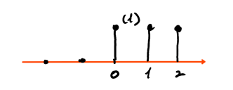
The DT unit step signal is a signal that is zero at negative values, and ones otherwise:

\begin{align} u[n] = \begin{cases} 0 & n < 0 \\ 1 & n \geq 0 \\ \end{cases} \end{align}

The plot for this is:

Signals can be either delayed:

\begin{align} \hat{\delta}[n] = \delta[n-1] \notag \end{align}

or advanced:

\begin{align} \tilde{\delta}[n] = \delta[n+1] \notag \end{align}

Note that non-integer shifts of a DT signal is meaningless since DT signals only have integer domains. Using the Kronecker delta, signal shifts, and scaling, any DT signal can be represented.

A subspace is a subset \(\mathcal{S}\) of a vector space \(\mathcal{V}\) that is itself a vector space. To test that a space is a vector space, it is sufficient to just show that:

1. \(0\) is an element of \(\mathcal{S}\)
2. \(\mathcal{S}\) is closed under vector addition
3. \(\mathcal{S}\) is closed under scalar multiplication