Diodes
Table of Contents
1. PN Junction
A PN junction is formed by placing n-type (extra free electrons) and p-type (extra free holes) semiconductors next to one another. Then, due to diffusion, the holes in the p-type material wish to move towards the n-type material, and vice versa:
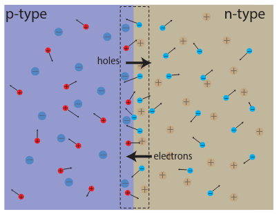
These mobile carriers become minority carriers in the new region. As the holes and free electrons move toward each other at the boundary, they recombined to form a depletion region where there are no charge carriers. What remains are the negative and positive ions, which form a electric field due to the difference in electric potential:
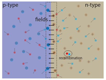
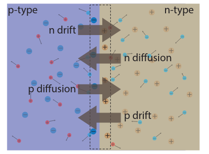
This electric field then causes a drift current in the opposite direction of diffusion (since electrons move opposite to electric field). When an electron-hole pair gets spontaneously generated in the region, the drift current pulls the electron towards the n-type and the hole towards the p-type. In steady state, the drift and diffusion currents balance out with zero net current:
For the p-type side, the Fermi energy is low because you are less likely to find a free electron in the conduction band, and the opposite side for the n-type side. When we reach steady state, however, the Fermi energy must be constant between the n-side and the p-side, because otherwise we would have a gradient. Therefore, the conduction and valence bands bend across the junction, as shown below. Another way to think about this is that for an electron to move from the n-type side to the p-type side, it must obtain energy to cross the electric field. This change in potential across the two sides is called the built-in potential, \(q\psi_0\):
We know the electrons and holes follow the Boltzmann distribution, and so only the small amount of electrons/holes at the correct energy levels form the diffusion current. Simultaneously, free electron and holes in the depletion region are drawn to their respective sides due to drift current.
The built-in potential can be deconstructed as:
\begin{align} q\phi_{bi} &= q(\phi_p + \phi_n) \notag \\ &= (E_{i, p} - E_F) + (E_F - E_{i, n}) \notag \end{align}We know that at room temperature, \(n = N_D = n_i e^{\frac{E_f-E_i}{kT}}\), so \(E_F - E_{i, n} = kT \ln\left(\frac{N_D}{n_i}\right)\). Doing the same thing for \(p\) and substituting back into the previous equation, we get
\begin{align} \phi_{bi} = \frac{kT}{q}\ln\left(\frac{N_AN_D}{n_i^2}\right) \end{align}Here we see that our built-in potential scales proportional to the temperature it is at as well as the concentration of acceptors and donors.
1.1. External Biases
When we forward bias our PN junction, we introduce more electrons into the n-type area and more holes into the p-type area:
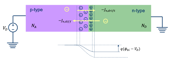
When we apply the forward bias, we apply an opposite electric field to the junction, which causes the barrier potential between the p-type side and n-type side to drop. Now, more electrons are able to flow from one side to the other, which increases our diffusion current. At the same time, we have also reduced the size of our depletion region, which reduces our drift current (since electric field is weaker):
On the other hand, if we reverse bias our PN junction, much of the opposite happens:
The Boltzmann distribution for carrier concentration allows us to say that the diffusion current when \(V_D = 0\) is directly proportional to \(e^{-\frac{q\phi_{bi}}{kT}}\), and that the diffusion current when \(V_D \neq 0\) is directly proportional to \(e^{-\frac{q(\phi_{bi}-V_D)}{kT}}\). Then, the actual current as a function of voltage is the difference between these two (difference between biased current and non-biased current):
\begin{align} I(V) &\propto e^{-\frac{q(\phi_{bi}-V_D)}{kT}} - e^{-\frac{q\phi_{bi}}{kT}} \notag \\ &\propto e^{-\frac{q\phi_{bi}}{kT}}\left(e^{\frac{qV_D}{kT}} - 1\right) \notag \end{align}Adding in our proportionality constant \(I_s\), we can write:
\begin{align} \boxed{I(V) = I_s\left(e^{\frac{qV_D}{kT}} - 1\right)} \end{align}This then gives us our diode I-V curve:
The tail on the left side of the plane is our saturation current as \(V_D\) goes very negative; this area becomes dominated by drift current, since as our depletion region grows bigger and bigger our diffusion current goes to zero. Similarly, the right side of the plane is dominated by diffusion current as the depletion region becomes smaller and smaller.
We can calculate \(I_S\) using the following relationship:
\begin{align} I_S = qn_i^2\left(\frac{D_n}{L_nN_a}+\frac{D_p}{L_pN_d}\right)A \end{align}where \(A\) is cross sectional area, and \(L_p\) and \(L_n\) are the minority carrier diffusion lengths (the average distance a minority carrier travels via diffusion before recombination occurs).
1.2. Junction Capacitance
At the PN junction, we have some negative charge and some positive charge that are separated. This means that we have some amount of capacitance at the boundary. We call that capacitance per unit area the junction capacitance \(C_j = \frac{C}{A}\).
Let the length of the p-type depletion region be \(x_p\), and the length of the n-type depletion region be \(x_n\). We can graph the charge concentration \(\rho\) of the junction like so:
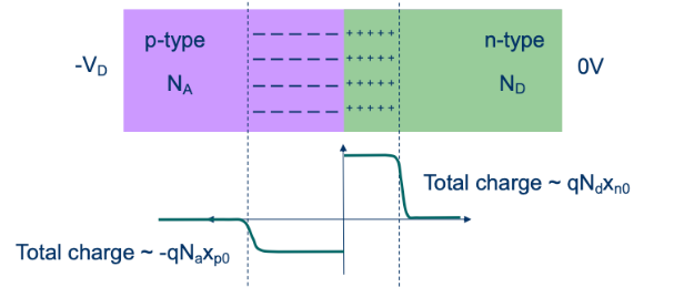
We can say that the total charge on both sides is equal. This is because the amount of charged ions left behind, say in the p-type region, is equal to the number of holes that have recombined with the free electrons from the n-type region. Therefore, we can write the following relationship:
\begin{align} x_pN_A = x_nN_D \notag \\ &\Rightarrow x_p+x_n = x_n\left(\frac{N_A+N_D}{N_A}\right) \notag \\ &\Rightarrow N_Dx_n = \frac{(x_p+x_n)N_DN_A}{N_D+N_A} \notag \end{align}Gauss’s law tells us that \(\mathbf{E} = \frac{1}{\epsilon_s} \int{\rho}\text{ d}x\), so we can graph the electric field like so:

The maximum electric field point \(E_{\text{max}} = \frac{qN_Ax_p}{\epsilon_s} = \frac{qN_Dx_n}{\epsilon_s}\). Substituting the relationship we got for \(N_dx_n\) earlier, we find that the max electric field is:
\begin{align} \boxed{E_{\text{max}} = \frac{q}{\epsilon_s}\left(\frac{N_AN_D}{N_A+N_D}\right)(x_p+x_n)} \end{align}Next, we know that \(E = -\nabla \phi \Rightarrow \phi = -\int E\text{ d}x\), where \(\phi\) is potential. Therefore, \(\phi_n = \frac{E_{\text{max}}x_n}{2}\) and \(\phi_p = \frac{E_{\text{max}}x_p}{2}\), taking the area of the triangle regions. Adding these two terms up gives us the total built-in potential, which can be written as:
\begin{align} \phi_{bi} - V_D &= \frac{E_{\text{max}}}{2}(x_n+x_p) \notag \\ &= \frac{q}{2\epsilon_s}\frac{N_AN_D}{N_A+N_D}(x_n+x_p)^2 \notag \end{align}Defining \(x_d = x_n+x_p\), we find that:
\begin{align} \boxed{x_d = \sqrt{\frac{2\epsilon_s}{q}\left(\frac{N_A+N_D}{N_AN_D}\right)(\phi_{bi}-V_D)}} \end{align}Plugging this back into our equation for junction capacitance, we finally get that
\begin{align} \boxed{C_j = \left[\frac{q\epsilon_s}{2\left(\frac{1}{N_A}+\frac{1}{N_D}\right)(\phi_{bi} - V_D)}\right]^{\frac{1}{2}} = \frac{C_{j_0}}{\sqrt{1-\frac{V_D}{\phi_{bi}}}}} \end{align}where \(C_{j_0}\) is \(C_j\) when \(V_D=0\). \(x_d\) is dominated by the side that is lightly doped.
2. Diode Small-Signal Model
The small-signal model for a diode in forward bias consists of a current source in parallel with a resistance, junction capacitance, and diffusion capactiance:
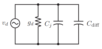
The parallel resistance \(g_d\) is:
\begin{align} g_d = \frac{qI}{kT} \end{align}And the diffusion capacitance \(C_{\text{diff}}\) is:
\begin{align} C_{\text{diff}} = \left(\frac{qI}{kT}\right) \tau_F \end{align}where \(\tau_F\) is a time constant that measures the time to cross the junction. Diffusion capacitance is caused by the diffusion of excess minority carriers as they wait to recombine.