Symmetric Matrices

1. Symmetric Matrices
- 1.1. Diagonalization
- 1.2. Spectral Decomposition
2. Quadratic Forms
- 2.1. Change of Variable
- 2.2. Classifying Quadratic Forms

1. Symmetric Matrices

A real square matrix \(S\) is called symmetric if:

\begin{align} S^T = S \end{align}

Looking at their eigenvalues and eigenvectors, we can see why they are special:

All \(n\) eigenvalues \(\lambda\) of a symmetric matrix are real numbers.
Each eigenvalue has algebraic multiplicity = geometric multiplicity.
The \(n\) eigenvectors can be chosen orthogonal to each other.

Why must they be orthogonal to each other? Consider two distinct eigenvalues \(\lambda_1\) and \(\lambda_2\), with their corresponding eigenvectors being \(\mathbf{v}_1\) and \(\mathbf{v}_2\). Then, consider:

\begin{align} \lambda_1 \mathbf{v}_1^T\mathbf{v}_2 &= \lambda_1(\mathbf{v}_1 \cdot\mathbf{v}_2) \notag \\ &= (\lambda_1\mathbf{v}_1)^T\mathbf{v}_2 \notag \\ &= (A\mathbf{v}_1)^T\mathbf{v}_2 \notag \\ &= \mathbf{v}_1^TA^T\mathbf{v}_2 \notag \\ &= \mathbf{v}_1^TA\mathbf{v}_2 \notag \\ &= \lambda_2\mathbf{v}_1^T\mathbf{v}_2 \notag \end{align}

But since \(\lambda_1 \neq \lambda_2\), the only way for this equality to hold would be if \(\mathbf{v}_1^T\mathbf{v}_2 = 0 \Rightarrow \mathbf{v}_1 \cdot \mathbf{v}_2 = 0\).

The other case is if we have repeated eigenvalues. However, if we have repeated eigenvalues that do not yield orthogonal eigenvectors, we can simply apply Gram-Schmidt to get orthogonal eigenvectors for that eigenspace.

1.1. Diagonalization

A symmetric matrix \(S\) is orthogonally diagonalizable, which means that there exists matrices \(Q\) and \(\Lambda\) such that \(\Lambda\) is diagonal and \(Q\) is an orthogonal matrix:

\begin{align} \boxed{S = Q\Lambda Q^T} \end{align}

We see that every matrix of this form is symmetric: taking the transpose of the diagonalization, we get \(Q^{TT}\Lambda^TQ^T = Q\Lambda Q^T\).

1.2. Spectral Decomposition

The three properties listed at the top lead to an interesting breakdown of the symmetric matrix, known as the spectral decomposition. If \(S\) is a symmetric matrix with eigenvalues \(\lambda_1, \lambda_2, \dots , \lambda_n\) and orthonormal eigenvectors \(\mathbf{u}_1, \mathbf{u}_2, \dots, \mathbf{u}_n\), then:

\begin{align} \boxed{S = \lambda_1\mathbf{u}_1\mathbf{u}_1^T + \lambda_2\mathbf{u}_2\mathbf{u}_2^T +\cdots + \lambda_n\mathbf{u}_n\mathbf{u}_n^T} \end{align}

We can see why this is true if we multiply both sides on the right by \(\mathbf{u}_1\). Then, all the terms on the right hand side of the equation go to zero since they are orthogonal to \(\mathbf{u}_1\), except for \(\lambda_1\mathbf{u}_1\mathbf{u}_1^T\). Thus we have \(S\mathbf{u}_1 = \lambda_1\mathbf{u}_1\), which is true by the definition of eigenvectors.

2. Quadratic Forms

For an \(n \times n\) symmetric matrix \(S\), given a vector \(\mathbf{x} \in \mathbb{R}^n\), define the quadratic form as the function \(Q: \mathbb{R}^n \rightarrow \mathbb{R}\):

\begin{align} \boxed{Q(\mathbf{x}) = \mathbf{x}^TS\mathbf{x}} \end{align}

where \(S\) is known as the matrix of the quadratic form.

We can write the quadratic form out generally for a \(2 \times 2\) symmetric matrix:

\begin{align} \begin{bmatrix} x_1 & x_2 \end{bmatrix} \begin{bmatrix} a & b \\ b & c \end{bmatrix} \begin{bmatrix} x_1 \\ x_2 \end{bmatrix} &= \begin{bmatrix} x_1 & x_2 \end{bmatrix} \begin{bmatrix} ax_1 + bx_2 \\ bx_1 + cx_2 \end{bmatrix} \notag \\ &= ax_1^2 + bx_1x_2 + bx_1x_2 + cx_2^2 \notag \\ &= ax_1^2 + 2bx_1x_2 + dx_2^2 \end{align}

2.1. Change of Variable

We see that above, we have a mixed term \(2bx_1x_2\), which complicates things. Fortunately, we can eliminate this mixed term by making a suitable change of variable with some \(n \times n\) invertible matrix \(P\):

\begin{align} \mathbf{x} = P\mathbf{y} \end{align}

Using this in the quadratic form, we get:

\begin{align} Q &= \mathbf{x}^TA\mathbf{x} \notag \\ &= (P\mathbf{y})^TA(P\mathbf{y}) \notag \\ &= \mathbf{y}^T(P^TAP)\mathbf{y} \notag \end{align}

Using the \(2 \times 2\) matrix above as an example, we see that in order to eliminate the mixed term, we want the matrix product \(P^TAP\) to be a diagonal matrix. Since \(A\) is symmetric, we can orthogonally diagonalize it with some orthogonal matrix \(P\) and diagonal matrix \(D\):

\begin{align} A &= PDP^T \notag \\ \Rightarrow P^TAP &= D \notag \end{align}

Thus, we can use the same \(P\) as in our diagonalization of \(A\) in the change of variables equation in order to get a quadratic form with no mixed terms.

2.2. Classifying Quadratic Forms

The quadratic form \(Q\) can be viewed as a real function. If \(A\) is a \(2 \times 2\) matrix, then we have several possibilities, where \(z = Q(\mathbf{x})\):

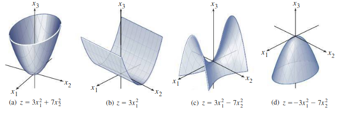
We can then classify \(Q\) based on the sign it takes on. A quadratic form \(Q\) is:

positive definite if \(Q(\mathbf{x}) > 0 \; \forall \: \mathbf{x} \neq 0\),
negative definite if \(Q(\mathbf{x}) < 0 \; \forall \: \mathbf{x} \neq 0\),
positive semidefinite if \(Q(\mathbf{x}) \geq 0 \; \forall \: \mathbf{x}\),
negative semidefinite if \(Q(\mathbf{x}) \leq 0 \; \forall \: \mathbf{x}\),
indefinite if \(Q(\mathbf{x})\) assumes both negative and positive values.

In the example above, (a) and (b) are both positive semidefinite, but (a) is better described as positive definite.

Since with a change of variables \(\mathbf{x} = P\mathbf{y}\) we can write \(Q(\mathbf{x}) = \mathbf{y}^TD\mathbf{y}\), where \(D\) has the eigenvalues of \(A\) on the diagonal, we can relate these classifications to the eigenvalues of \(A\). The quadratic form \(Q\) is:

Positive definite if and only if the eigenvalues of \(A\) are all positive,
Negative definite if and only if the eigenvalues of \(A\) are all negative,
Indefinite if and only if \(A\) has both positive and negative eigenvalues.