Second-Order Circuits
Table of Contents
1. RLC Series Circuit
Consider the following RLC circuit in series:
Considering \(t \gg 0\), KVL gives us:
\begin{align} v_R + v_L + v_C &= v_0 \notag \\ IR + L\frac{\text{d}I}{\text{d}t} + v_C &= v_0 \notag \end{align}Since \(I=C\frac{\text{d}v_c}{\text{d}t}\), we have:
\begin{align} RC\frac{\text{d}v_C}{\text{d}t} + L\frac{\text{d}}{\text{d}t}\left[C\frac{\text{d}v_C}{\text{d}t}\right]+v_C &= v_0 \notag \\ RC\frac{\text{d}v_C}{\text{d}t} + LC\frac{\text{d}^2v_C}{\text{d}t^2}+v_C &= v_0 \notag \end{align}Dividing by \(LC\) and rearranging,
\begin{align} \frac{\text{d}^2v_C}{\text{d}t^2}+\frac{R}{L}\frac{\text{d}v_C}{\text{d}t}+\frac{v_C}{LC}=\frac{v_0}{LC} \notag \end{align}Therefore, we get the following second-order differential equation:
\begin{align} \boxed{\frac{\text{d}^2v_C}{\text{d}t^2} + 2\alpha\frac{\text{d}v_C}{\text{d}t}+\omega_0^2v_C = \omega_0^2v_0} \end{align}where \(\alpha = \frac{R}{2L}\) and \(\omega_0^2 = \frac{1}{LC}\).
2. RLC Parallel Circuit
Consider the following RLC circuit in parallel:
By KCL, we get:
\begin{align} i_R+i_L+i_C&=i_S \notag \\ \frac{v_R}{R} + i_L+C\frac{\text{d}v_C}{\text{d}t}&=i_S \notag \end{align}We know that \(v_R=v_L=v_C\), so
\begin{align} v_L=L\frac{\text{d}i_L}{\text{d}t}=v_C \notag \end{align}Then, substituting back into our original equation, we get
\begin{align} \frac{v_L}{R} + i_L + C\frac{\text{d}v_L}{\text{d}t} &= i_S \notag \\ \frac{L}{R}\frac{\text{d}i_L}{\text{d}t} + i_L + C\frac{\text{d}}{\text{d}t}L\frac{\text{d}i_L}{\text{d}t} &= i_S \notag \\ LC\frac{\text{d}^2i_L}{\text{d}t^2} + \frac{L}{R}\frac{\text{d}i_L}{\text{d}t} + i_L &= i_S \notag \\ \end{align}Dividing by \(LC\) and rearranging, we get the following differential equation:
\begin{align} \boxed{\frac{\text{d}^2i_L}{\text{d}t^2} + 2\alpha\frac{\text{d}i_L}{\text{d}t} + \omega_0^2i_L = \omega_0^2i_S} \end{align}where \(\alpha = \frac{1}{2RC}\) and \(\omega_0^2 = \frac{1}{LC}\).
3. Frequency Response of RLC Circuits
Solving for the homogenous response, we get the following results from the characteristic equation:
\begin{align} s = -\alpha \pm \sqrt{\alpha^2 - \omega_0^2} \end{align}Thus, the homogenous solution is of the form:
\begin{align} v_C(t) = A_1e^{s_1t}+A_2e^{s_2t} \end{align}Depending on \(\alpha\) and \(\omega_0\), we can get several different situations:
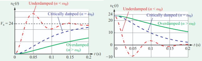
Example: Frequency response of RLC circuit
Consider the following RLC circuit:
We want to evaluate the response of this circuit for \(t \geq 0\), given that the circuit reaches steady state prior to \(t=0\). Then, our initial conditions are:
\begin{align} v_C(0) &= 24 \notag \\ i(0) &= 0 \notag \end{align}Now, we calculate that \(\alpha = 20\) and \(\omega_0=68\), so we are in the underdamped case. Our solution looks like this:
\begin{align} v_C(t) = \left(A_1\cos(\omega_dt)+A_2\sin(\omega_dt)\right)e^{-\alpha t} + v_C(t\rightarrow \infty) \notag \end{align}Since \(\omega_d=\sqrt{\omega_0^2 -\alpha^2} = 65\) and \(v_C(t\rightarrow\infty)=0\), we have:
\begin{align} v_C(t) = \left(A_1\cos(65t)+A_2\sin(65t)\right)e^{-20t} \notag \end{align}Applying the initial conditions,
\begin{align} v_C(0) &= 24 = A_1 \notag \\ i(0) &= 0 = C\frac{\text{d}v_C}{\text{d}t} \notag \\ &= C\left(\left[65A_2\cos(65t)-65A_1\sin(65t)\right]e^{-20t}-20e^{-20t}\left[A_1\cos(65t)+A_2\sin(65t)\right]\right) \notag \\ &= C(65A_2-20A_1) \Rightarrow A_2=7.38 \notag \end{align}Thus, the solution is:
\begin{align} v_C(t) = \left[24\cos(65t)+7.38\sin(65t)\right]e^{-20t} \notag \end{align}3.1. Overdamped
When \(\alpha > \omega_0\), the term under the square root (\(\alpha^2 - \omega_0^2\)) is strictly positive. This means the roots of the characteristic equation, \(s_1\) and \(s_2\), are both real, distinct, and negative.
The homogenous response is simply the sum of two decaying exponentials:
\begin{align} v_C(t) = A_1e^{s_1t} + A_2e^{s_2t} \notag \end{align}Because \(s_1\) and \(s_2\) are strictly negative, this can also be explicitly written using absolute values as \(v_C(t) = A_1e^{-|s_1|t} + A_2e^{-|s_2|t}\). This is known as an overdamped circuit, as it slowly decays to the steady-state equilibrium without oscillating.
3.2. Underdamped
When \(\alpha < \omega_0\), the term under the square root is negative, leading to complex conjugate roots. We can define the damped resonant frequency, \(\omega_d\), to handle the negative square root:
\begin{align} \omega_d = \sqrt{\omega_0^2 - \alpha^2} \notag \end{align}The roots then become \(s = -\alpha \pm j\omega_d\). Substituting these into our homogenous solution gives:
\begin{align} v_C(t) &= A_1e^{(-\alpha + j\omega_d)t} + A_2e^{(-\alpha - j\omega_d)t} \notag \\ &= e^{-\alpha t}\left[A_1e^{j\omega_dt} + A_2e^{-j\omega_dt}\right] \notag \end{align}To convert this into a strictly real function, we use Euler’s formula:
\begin{align} v_C(t) &= e^{-\alpha t} \left[ A_1(\cos\omega_dt + j\sin\omega_dt) + A_2(\cos\omega_dt - j\sin\omega_dt) \right] \notag \\ &= e^{-\alpha t} \left[ (A_1 + A_2)\cos\omega_dt + j(A_1 - A_2)\sin\omega_dt \right] \notag \\ &= e^{-\alpha t} \left[ B_1\cos(\omega_dt) + B_2\sin(\omega_dt) \right] \notag \end{align}where our new, entirely real constants are defined as:
- \(B_1 = A_1 + A_2\)
- \(B_2 = j(A_1 - A_2)\)
This is an underdamped circuit. The \(e^{-\alpha t}\) envelope causes the amplitude to decay exponentially, while the sinusoidal terms cause the voltage to oscillate as it decays.
3.3. Critically Damped
When \(\alpha = \omega_0\), the term under the square root is exactly zero. This gives us a single repeated real root:
\begin{align} s_1 = s_2 = -\alpha \notag \end{align}We need to multiply the second solution by \(t\) to form a set of two linearly independent solutions. Therefore, the homogenous response is:
\begin{align} v_C(t) = A_1e^{-\alpha t} + A_2te^{-\alpha t} \notag \end{align}or, factored out:
\begin{align} v_C(t) = (A_1 + A_2t)e^{-\alpha t} \notag \end{align}This is called a critically damped circuit. It represents the precise boundary between oscillating (underdamped) and non-oscillating (overdamped) responses. A critically damped system provides the fastest possible return to equilibrium without any overshoot.
3.4. Undamped (Resonance)
As a special condition, consider an ideal LC circuit where the resistance \(R = 0\). Since \(\alpha = \frac{R}{2L}\), this means the damping factor \(\alpha = 0\).
The roots of the characteristic equation lose their real component and become purely imaginary:
\begin{align} s = \pm j\omega_0 \notag \end{align}Substituting this into the underdamped equation (where the exponential decay term \(e^{-\alpha t} = e^0 = 1\)), we get:
\begin{align} v_C(t) &= A_1e^{j\omega_0t} + A_2e^{-j\omega_0t} \notag \\ &= B_1\cos\omega_0t + B_2\sin\omega_0t \notag \end{align}Because there is no resistance to dissipate energy, the circuit experiences no exponential decay. It oscillates perpetually as a pure sine wave at its natural resonant frequency, \(\omega_0\). This state is known as an undamped response or resonance.