MOSFETs
Table of Contents
1. MOS Capacitor
A metal oxide semiconductor (MOS) capacitor is composed of a metal (conductor) layer, an oxide (insulator) layer, and a semiconductor layer. Say the semiconductor layer is p-type, and that it acts somewhat like a metal: we now have something that looks like a capacitor:
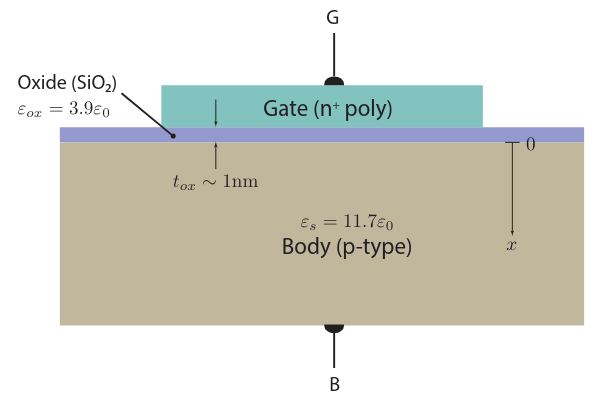
We can draw the band diagram for a metal, oxide, and p-type semiconductor like so:
where \(\Phi\) is the work function, the minimum amount of energy required for an electron at the Fermi level to leave the specific material and go to free space, and \(\chi\) is the electron affinity, the difference between the vacuum band energy and conduction band energy.
From this diagram we can also write down a formula for the work function of the semiconductor:
\begin{align} \Phi_s = \chi_s + (E_c - E_f) \notag \end{align}We are going to first make two assumptions that we shall come back to later:
- There are no net charges in the oxide material, or at the oxide-semiconductor interface.
- Flat-band assumption: \(\Phi_m=\Phi_s\), or in other words the Fermi level is the same for the metal and the semiconductor.
Now, we can join the metal, oxide, and semiconductor band diagrams together to give the following combined band diagram with no voltage applied at the gate, using a box to denote the oxide and emphasize the separation between the layers:
1.1. Accumulation
Say we now apply a negative voltage to the gate (with the body grounded), i.e. \(V_G < 0\). Then, negative charges build up at the metal-oxide interface, and there are plenty of holes in the p-type material to flow toward the negative charges at the semiconductor-oxide interface. There is now an electric field across the oxide material, and we call this the accumulation mode:
The MOSCAP in accumulation mode acts as a capacitor: it has a constant electric field across the oxide (since we assume no charge within the oxide).
1.2. Depletion
Now let’s say \(V_G>0\) (and below some threshold). As we apply the voltage, positive charges will flow to the gate (i.e. electrons will leave the gate). This will then repel the holes which form the majority carrier in the p-type semiconductor, leaving behind negative ions. These negative ions form a depletion region, putting the MOSCAP into depletion mode:
1.3. Inversion
Once we increase the gate voltage past some voltage \(V_T\), we reach inversion. Here, the minority carriers (e.g. electrons for p-type semiconductor) get attracted to the oxide boundary and form an inversion layer:
Notice that at the inversion layer, the conduction band energy is closer to the Fermi energy level than the valence band: at this layer, we have formed an n-type region inside of our p-type region! The point where the difference between the intrinsic energy level and the Fermi energy level at the inversion layer is the same as in the p-type region is called strong inversion: this is where the inversion layer looks as much like an n-type as the semiconductor looks like a p-type. The \(V_T\) at which we reach strong inversion is called the threshold voltage.
Define \(\Delta E_1 = E_f - E_i\) at the surface (inversion layer) and \(\Delta E_2 = E_i - E_f\) in the bulk, so that both are positive. We know that due to carrier distribution, the electron concentration at the surface and the hole concentration in the bulk are
\begin{align} n_s &= n_i e^{\frac{E_f-E_i}{kT}} = n_i e^{\frac{\Delta E_1}{kT}} \notag \\ p_0 &= n_i e^{\frac{E_i-E_f}{kT}} = n_i e^{\frac{\Delta E_2}{kT}} \notag \end{align}At strong inversion, \(\Delta E_1 = \Delta E_2 = q\phi_f\). So, another way of thinking about strong inversion is that it is the point where the concentration of minority carriers in the inversion layer is the same as the concentration of majority carriers in the rest of the semiconductor. We can then write
\begin{align} n_s=p_0= n_i e^{\frac{q\phi_f}{kT}} \end{align}1.3.1. Derivation of Threshold Voltage
In order to derive the threshold voltage, then, we would like to find these concentrations as a function of the applied gate voltage. We can express \(V_G\) as two terms, the voltage/potential drop from the oxide interface across the semiconductor \(\phi_s\), and the change in voltage across the oxide \(\Delta \phi_{\text{ox}}\):
\begin{align} V_G = \phi_s + \Delta \phi_{\text{ox}} \notag \end{align}\(\phi_s\) is also called the surface potential. Say \(x=0\) at the oxide-semiconductor surface, and we call \(x=x_d\) the edge of the depletion region, where \(\mathcal{E}=0\) and \(\phi=0\). From Gauss’s Law, we can find the electric field as a function of distance for \(0 \le x \le x_d\):
\begin{align} \mathcal{E}(x) = \frac{qN_A}{\epsilon_s}(x_d-x) \notag \end{align}Then the potential function is the negative integral of the electric field:
\begin{align} \phi(x) = -\int_{x_d}^x \mathcal{E}(x)\text{ d}x = \frac{qN_A}{2\epsilon_s}(x-x_d)^2 \notag \end{align}The surface potential is just the potential when \(x=0\), so we get:
\begin{align} \phi_s = \frac{qN_Ax_d^2}{2\epsilon_s} \end{align}Now for the potential across the oxide. This is easier to find since we have a constant electric field:
\begin{align} \Delta \phi_{\text{ox}} = t_{\text{ox}}\mathcal{E}_{\text{ox}} \end{align}where \(t_{\text{ox}}\) is the thickness of the oxide layer. At the boundary, the electric displacement must satisfy this continuity equation:
\begin{align} \epsilon_{\text{ox}}\mathcal{E}_{\text{ox}} = \epsilon_s\mathcal{E}_s \notag \end{align}where \(\mathcal{E}_s = \mathcal{E}(0) = \frac{qN_Ax_d}{\epsilon_s}\). Therefore, we can rewrite (3) to be:
\begin{align} \Delta\phi_{\text{ox}} = t_{\text{ox}}\mathcal{E}_s\frac{\epsilon_s}{\epsilon_{\text{ox}}} = \frac{t_{\text{ox}}}{\epsilon_{\text{ox}}}qN_Ax_d = \frac{qN_Ax_d}{C_{\text{ox}}} \notag \end{align}We define \(C_{\text{ox}} = \frac{\epsilon_{\text{ox}}}{t_{\text{ox}}}\), which is the capacitance per unit area for the oxide.
From (2) we can see that \(qN_Ax_d = \sqrt{2\epsilon_s qN_A\phi_s}\). Plugging this in to our equation yields
\begin{align} \Delta\phi_{\text{ox}} = \frac{\sqrt{2\epsilon_sqN_A}}{C_{\text{ox}}}\sqrt{\phi_s} = \gamma\sqrt{\phi_s} \notag \end{align}Therefore, we can now write:
\begin{align} V_G = \phi_s + \gamma\sqrt{\phi_s} \notag \end{align}Now, say that the Fermi potential of the bulk semiconductor is \(\phi_f\), where \(q\phi_f = E_i - E_f = \Delta E_2\). Then the surface potential (the voltage drop across the entire semiconductor) at strong inversion is \(\phi_s = 2\phi_f\), since the bands must bend by \(\Delta E_2\) to bring \(E_i\) down to \(E_f\) at the surface, and then by a further \(\Delta E_1 = \Delta E_2\) to reach strong inversion. Therefore, \(V_G\) at strong inversion is the threshold voltage:
\begin{align} V_{T_0} = 2\phi_f + \gamma\sqrt{2\phi_f} \notag \end{align}where \(\phi_f = \frac{kT}{q}\ln\left(\frac{N_A}{n_i}\right)\).
Now, let’s revisit our assumptions. We can no longer assume that our work functions are equal, or that there is no charge in the oxide, so we must apply a correction to make the bands flat. This correction is called \(V_{FB}\), or the flat-band voltage:
\begin{align} V_{FB} = \frac{\Phi_m - \Phi_s}{q} - \frac{Q_{\text{ox}}}{C_{\text{ox}}} \notag \end{align}Thus, our final threshold voltage is:
\begin{align} \boxed{V_T = V_{FB} + 2\phi_f + \gamma\sqrt{2\phi_f}} \end{align}where \(\gamma = \frac{\sqrt{2\epsilon_sqN_A}}{C_{\text{ox}}}\).
2. MOSFET
The metal-oxide-semiconductor field-effect transistor, or MOSFET, is a kind of voltage-controlled current source. A MOSFET consists of a doped semiconductor substrate, above which there is an oxide, and a metal gate (much like a MOS capacitor). Additionally, however, we introduce two wells:
When we apply a large gate voltage, similar to what happens during inversion, a layer of minority carriers form at the oxide interface. These minority carriers are now quickly supplied by the wells: when you increase the gate voltage, electrons pour into the substrate from the wells and form a channel; when you decrease the gate voltage, electrons escape back into the wells. The above is example for an n-channel MOSFET.
Usually, the well that is grounded is called the source terminal, and the other the drain terminal. Along with the gate, we also sometimes define the body terminal which connects to the body or the bulk semiconductor substrate.
Additionally, we must also consider the PN junctions that are formed by source/drain and the body. We don’t want current flowing from source/drain into the body, and thus it is in our interest to keep these junctions reverse biased. To do so, the potential of the body should not be higher than that of source or drain.
The voltage of the body affects the formation of the channel, thus, the threshold voltage is also affected by \(V_{BS}\). This effect of having a voltage between body and source changing the threshold voltage is called the body effect:
\begin{align} \boxed{V_T = V_{FB} + 2\phi_f + \gamma\sqrt{2\phi_f + V_{\text{SB}}}} \end{align}2.1. MOSFET Symbol
3. MOSFET Operating Regions
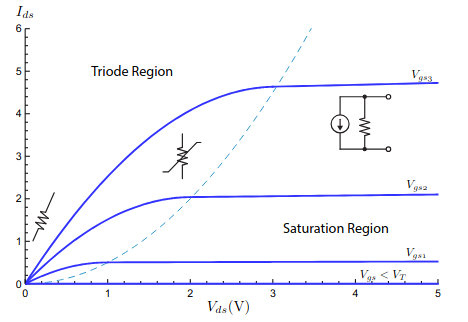
If we graph the current-voltage relationship of a MOSFET, we can split it up into several operating regions:
3.1. Linear/Triode
When \(V_{\text{GS}} > V_T\), the inversion channel forms and charge can flow. The total charge in the channel is given by capacitance. For small \(V_{\text{DS}}\), we are operating in the linear region, and we can approximate the channel as a rectangle with length \(L\):
\begin{align} q_{\text{ch}} &= C(V_{\text{GS}}-V_T) \notag \\ &= C_{\text{ox}}WL(V_{\text{GS}}-V_T) \notag \end{align}Current is charge per unit time. The time it takes for all that charge to cross the channel is:
\begin{align} \tau = \frac{L}{v_d} = \frac{L}{\mu_nE} = \frac{L}{\mu\frac{V_{\text{DS}}}{L}} = \frac{L^2}{\mu_nV_{\text{DS}}} \notag \end{align}Thus, the drain current is just \(\frac{q_{\text{ch}}}{\tau}\):
\begin{align} \boxed{I_D = \mu_nC_{\text{ox}}\frac{W}{L}(V_{\text{GS}}-V_T)V_{\text{DS}}} \end{align}However, for larger \(V_{\text{DS}}\), we cannot apprximate the channel as “flat.” That is, when \(V_{\text{GS}} > V_T\) but \(V_{\text{DS}} < V_{\text{GS}}-V_T\), which is commonly referred to as the triode region. Instead, since we are also applying a voltage to drain, the inversion region “bends” like so:
This is because the applied voltage also attracts electrons in the horizontal direction, which decreases the channel width. Then, we must use calculus to find the drain current:
\begin{align} I_D &= \frac{\text{d}q}{\text{d}\tau} \notag \\ &= \frac{WC_{\text{ox}}\text{d}x[V_{\text{GS}}-V_T-V(x)]}{\frac{\text{d}x}{\mu_n\text{d}V}} \notag \\ &= \mu_nC_{\text{ox}}W[V_{\text{GS}}-V_T-V(x)]\frac{\text{d}V}{\text{d}x} \notag \end{align}Multiplying by \(\text{d}x\) and taking the integral, we get:
\begin{align} \boxed{I_D = \mu_nC_{\text{ox}}\frac{W}{L}\left[(V_{\text{GS}}-V_T)V_{\text{DS}}-\frac{V_{\text{DS}}^2}{2}\right]} \end{align}3.2. Saturation
At saturation, the drain to source voltage rises high enough such that pinch-off occurs, where the channel length becomes shorter:
Current is still able to flow across the transistor due to the strong electric field between the end of the channel and the drain. However, at this point, the effective drain to source voltage at the end of the channel becomes fixed at \(V_{\text{GS}}-V_T\). Plugging this voltage for \(V_{\text{DS}}\) into our current for the triode region, we find that at saturation when \(V_{\text{DS}}>V_{\text{GS}}-V_T\), we have
\begin{align} I_D = \frac{1}{2}\mu_nC_{\text{ox}}\frac{W}{L_{\text{eff}}}(V_{\text{GS}}-V_T)^2 \notag \end{align}where \(L_{\text{eff}}\) is the effective length of the channel, since we have pinch-off. This length actually changes slightly as \(V_{\text{DS}}\), which is called channel length modulation. Thus, to actually use \(L_{\text{eff}}\) in our equation, we encode it into a constant \(\lambda\):
\begin{align} \boxed{I_D = \frac{1}{2}\mu_nC_{\text{ox}}\frac{W}{L}(V_{\text{GS}}-V_T)^2(1+\lambda V_{\text{DS}})} \end{align}\(\lambda\) is the slope of the curve when it is in the saturation region. Since the slope is \(I_D\) over \(V_{\text{DS}}\), multiplying it by \(V_{\text{DS}}\) gives us how much correction to the current we need.
4. MOSFET Small Signal Model
A small signal model attempts to linearize the behavior of a device around some bias point. We wish to linearize the behavior of a MOSFET around some \(V_{\text{GS}}\). Define transconductance \(g_m\) as
\begin{align} g_m = \frac{\partial I_D}{\partial V_{\text{GS}}} = \mu_n C_{\text{ox}}\frac{W}{L}(V_{\text{GS}}-V_T) = \sqrt{2\mu_n C_{\text{ox}} \frac{W}{L}I_D} = \frac{2I_D}{V_{\text{GS}}-V_T} \end{align}We ignore channel length modulation and small changes in \(V_{\text{GS}}\) here. We also need to account for \(I_D\) changing with \(V_{\text{DS}}\):
\begin{align} r_o = \left(\frac{\partial I_D}{\partial V_{\text{DS}}}\right)^{-1} = \frac{1}{\frac{1}{2}\mu_n C_{\text{ox}}\frac{W}{L}(V_{\text{GS}}-V_T)^2\lambda} = \frac{1}{\lambda I_D} \end{align}Then, the simplest small signal model of a MOSFET is:
From (5), however, \(I_D\) also depends on \(V_{\text{BS}}\). This is called body effect. So, we also want to know how \(I_D\) changes with \(V_{\text{BS}}\):
\begin{align} g_{mb} &= \frac{\partial I_D}{\partial V_{\text{BS}}} \notag \\ &= -\mu_n C_{\text{ox}} \frac{W}{L}(V_{\text{GS}} - V_T)\frac{\partial V_T}{\partial V_{\text{BS}}} \notag \\ &= \frac{g_m \gamma}{2\sqrt{2\phi_f + V_{\text{SB}}}} \notag \\ &= \frac{g_m\sqrt{2\epsilon_s q N_A}}{2\sqrt{2\phi_f + V_{\text{SB}}}C_{\text{ox}}} \notag \end{align}Taking the ratio of \(g_{mb}\) to \(g_m\), we get
\begin{align} \frac{g_{mb}}{g_m} &= \frac{\sqrt{2\epsilon_s q N_A}}{2\sqrt{2\phi_f + V_{\text{SB}}}C_{\text{ox}}} \notag \\ &= \frac{1}{C_{\text{ox}}}\sqrt{\frac{\epsilon_s q N_A}{2(2\phi_f+V_{\text{SB}})}} \notag \\ &= \frac{1}{C_{\text{ox}}}\epsilon_s\sqrt{\frac{q N_A}{2\epsilon_s(2\phi_f+V_{\text{SB}})}} \notag \end{align}Earlier, we found that \(x_d = \sqrt{\frac{2\epsilon_s V}{qN_A}}\). Then, \(\frac{g_{mb}}{g_m} = \frac{1}{C_{\text{ox}}}\frac{\epsilon_s}{x_{\text{sub}}}\), and
\begin{align} \frac{g_{mb}}{g_m} = \frac{C_{\text{sub}}}{C_{\text{ox}}} \end{align}We can think of this as a capacitor across the oxide and a capacitor across the substrate. Both capacitors are competing to accumulate charge in the channel, which is why the conductances are related to the capacitances. We want the oxide capacitor to be relatively large so that changing the gate to source voltage is effective at modulating charge in the channel. Now, our small signal model looks like this:
Taking it a step further, we also have to consider the capacitances between the different types of semiconductors in the transistor. From the junction capacitance of PN junctions, we can define the capacitance between source and base as well as between drain and base:
\begin{align} C_{sb} &= \frac{C_{{sb}_0}}{\sqrt{1+\frac{V_{\text{SB}}}{\phi_0}}} \\ C_{db} &= \frac{C_{{db}_0}}{\sqrt{1+\frac{V_{\text{DB}}}{\phi_0}}} \end{align}\(C_{{sb}_0}\) and \(C_{{db}_0}\) are the total zero-bias junction capacitances. They are calculated from the geometry of the MOSFET:
\begin{align} C_{\text{sb}_0} = C_{\text{db}_0} = \underbrace{C_{j0}\,W L_j}_{\text{bottom (area)}} \;+\; \underbrace{C_{jsw0}\,(W + 2L_j)}_{\text{sidewalls (perimeter)}} \end{align}There is also capacitance between gate and source, as well as between gate and drain:
\begin{align} C_{gs} &= WL_{ov}C_{\text{ox}} + \frac{2}{3}WLC_{\text{ox}} \\ C_{gd} &= WL_{ov}C_{\text{ox}} + C_{\text{fringe}} \end{align}\(C_{\text{fringe}}\) is the extra capacitance due to electric field lines that curve around the gate instead of going through the oxide. Adding these capacitors brings our small signal model to:
This model is known as the \(\pi\) model.
4.1. T Model
If we remove the current sources where they are at currently, and instead feed them through gate and body like so:
Note that this is fine since no current is actually entering the gate and body, they are being siphoned away fully. Then, we can transform this into the T small signal model: