Flux

If \(\vec{F}\) is a velocity field, then flux measures how much passes through a curve per unit time. If we consider really small segments of \(C\) with length \(\Delta s\), then we can model the total amount that passes through this segment as a parallelogram like so:

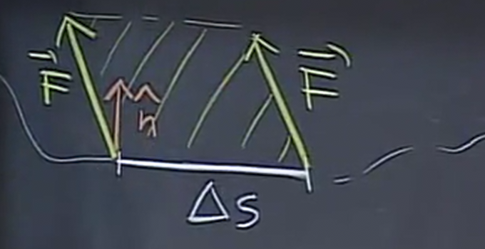
Now, to calculate the area, it is just the base times the height, where the height is the projection of \(\vec{F}\) onto \(\hat{n}\):

\[ A = \Delta s (\vec{F} \cdot \hat{n}) \]

Then, the sum of all of these segments of \(C\) gives us the line integral. The convention is that what flows across \(C\) left to right is positive, and what flows right to left is negative.

We know that \(\text{d}s\) is the scalar of \(\text{d}r\) from the line integral for work, so we can say that \(\text{d}r = \hat{T}\text{ d}s = \langle \text{d}x, \text{d}y \rangle\), where \(\hat{T}\) is the tangential unit vector. Since \(\hat{n}\) is simply \(\hat{T}\) rotated 90 degrees clockwise, we can say that

\[ \hat{n} \text{ d}s = \langle \text{d}y, -\text{d}x \rangle \]

Therefore, if \(\vec{F} = \langle P,Q \rangle\), we can express our line integral in component form as follows:

\[ \int_C P\text{ d}y - Q \text{ d}x \]

Then, applying Green's Theorem, where \(M=-Q\) and \(N=P\), we have:

\[ \oint_C P\text{ d}y - Q \text{ d}x = \iint_R (P_x + Q_y) \text{ d}A \]

Therefore, Green's Theorem for flux is:

\begin{align} \int_C \vec{F} \cdot \hat{n} \text{ d}s = \iint_R \text{div }\vec{F} \text{ d}A \end{align}

The divergence of \(\vec{F}\) is represented by \(\text{div }\vec{F} = P_x + Q_y\).

If a surface \(S\) is the graph of \(z=f(x,y)\), then we have the following expression:

\begin{align} \hat{n}\text{ d}S = \pm \langle -f_x.-f_y,1 \rangle \text{ d}x\text{ d}y \end{align}

We can prove this by considering a small section of the surface when we start at \((x,y,f(x,y))\) and change by tiny amounts \(\Delta x\) and \(\Delta y\). This results in a parallelogram shape, which we can find the area of by taking the cross product of the vectors of the two sides. This is also especially convenient because the cross product also returns the unit normal vector, which is exactly what we need.

Call the vector moving in the \(x\) direction \(\vec{u}\), and the vector moving in the \(y\) direction \(\vec{v}\). Then,

\begin{aligned} \vec{u} = \langle x+\Delta x, y, f(x+\Delta x, y)\rangle - \langle x,y,f(x,y) \rangle \\ \vec{v} = \langle x, y+\Delta y, f(x,y+\Delta y)\rangle - \langle x,y,f(x,y) \rangle \end{aligned}

Using linear approximation, we can rewrite \(f(x+\Delta x,y)\) to \(f(x,y) + \Delta xf_x\), and vice versa for \(\vec{v}\). Thus,

\begin{aligned} \vec{u} = \langle \Delta x, 0, f_x\Delta x \rangle = \langle 1,0,f_x \rangle \Delta x \\ \vec{v} = \langle 0, \Delta y, f_y\Delta y \rangle = \langle 0,1,f_y \rangle \Delta y \\ \end{aligned}

We can now do the cross product, which comes out to be:

\[ \vec{n}\Delta S = \vec{u} \times \vec{v} = \langle -f_x,-f_y,1 \rangle \Delta x \Delta y \]

Lots of times we want to do the surface integral if we know the normal vector \(\vec{N}\) to the surface. This occurs, for example, when we have a plane, or a function \(g(x,y,z)=0\) where we can obtain the normal vector through the gradient.

Consider the projection of the surface onto the xy plane, \(\Delta A\), and the angle it makes it with as \(\alpha\):

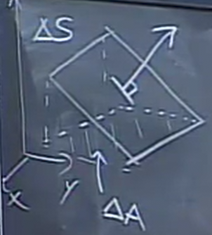
We can see that \(\Delta S = \cos \alpha \Delta A\). To find \(\cos \alpha\), consider that \(\alpha\) is also equivalent to the angle made between the normal vectors of the surface, \(\vec{N}\), and the projection, \(\hat{k}\). Thus:

\[ \Delta A = \Delta S \cos \alpha = \Delta S \frac{\vec{N}\cdot\hat{k}}{|\vec{N}|} \]

Then, \(\Delta S\) is:

\[ \Delta S = \frac{|\vec{N}|}{\vec{N} \cdot \hat{k}} \Delta A \]

Now, consider \(\hat{n}\Delta S\):

\[ \hat{n}\Delta S = \frac{|\vec{N}|\hat{n}}{\vec{N} \cdot \hat{k}} \Delta A = \pm \frac{\vec{N}}{\vec{N} \cdot \hat{k}} \Delta x \Delta y \]

Therefore, we can write that:

\begin{align} \hat{n}\text{ d}S = \pm \frac{\vec{N}}{\vec{N} \cdot \hat{k}} \text{ d}x\text{ d}y \end{align}