Oscillations

Systems that undergo simple harmonic motion can all be described with the canonical form for SHM:

\begin{align} \boxed{\frac{\text{d}^2x}{\text{d}t^2} + \omega^2x = 0} \end{align}

where \(\omega\) is the angular frequency in radians per second. Since all systems in SHM can be represented in this form, this leads us to find the following general solution for the position of a system in SHM:

\begin{align} \boxed{x(t) = A\cos(\omega t+\phi)} \end{align}

where \(A\) is the amplitude (which must be positive) and \(\phi\) is the phase shift in radians. The angular frequency is given based on which type of system is being analyzed, but \(A\) and \(\phi\) are determined based on initial values of the problem.

The spring-mass system undergoes SHM due to Hooke's Law, which tells us that the force is proportional to the spring's displacement:

From Newton's 2nd law, we can express the system in its canonical form:

\begin{align} -kx &= m\frac{\text{d}^2x}{\text{d}t^2} \notag \\ \frac{\text{d}^2x}{\text{d}t^2} + \frac{k}{m}x &= 0 \notag \end{align}

From this, we see that for a spring-mass system, the angular frequency is:

\begin{align} \boxed{\omega = \sqrt{\frac{k}{m}}} \end{align}

Example: Spring-mass system

Consider a block initially at rest after compressing a spring over a length \(L\), after which the system is released:

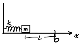
We want to find the final position of the block as a function of time. From the general solution:

\begin{align} x(t) = A\cos(\omega t + \phi), \: \omega = \sqrt{\frac{k}{m}} \notag \end{align}

Now we need to determine \(A\) and \(\phi\) from initial conditions. Since the system starts displaced by \(L\):

\begin{align} x(0) = A\cos\phi = -L \notag \end{align}

We also know that the system starts from rest, so taking the derivative to find the velocity gives:

\begin{align} v(t) &= -A\omega\sin(\omega t + \phi) \notag \\ v(0) &= -A\omega\sin\phi = 0 \notag \end{align}

Since \(A\) and \(\omega\) are both positive, this means that \(\sin \phi = 0\), giving us two possible values of \(\phi\): \(0\) and \(\pi\). Plugging these back into our first initial value equation, we find that the only solution that makes sense is \(\phi = \pi\) and \(A = L\). Thus, the position as a function of time for this system is:

\begin{align} \boxed{x(t) = -L\cos\left(\sqrt{\frac{k}{m}}t\right)} \notag \end{align}

The torsion pendulum consists of a system oscillating rotationally, like so:

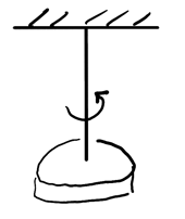
Its restoring torque can be found from a metaphor with Hooke's Law:

\begin{align} \tau = -\kappa\theta \end{align}

where \(\kappa\) is the torsional constant. We can write this in the canonical form by using Newton's 2nd law:

\begin{align} -\kappa\theta &= I\frac{\text{d}^2\theta}{\text{d}t^2} \notag \\ \frac{\text{d}^2\theta}{\text{d}t^2}+\frac{\kappa}{I}\theta &= 0 \notag \end{align}

Thus, from the canoncial form, we see that the angular frequency is:

\begin{align} \boxed{\omega = \sqrt{\frac{\kappa}{I}}} \end{align}

Note that for angular velocity, use \(\Omega(t)\) as the notation, since \(\omega\) would conflict with angular frequency.

The simple pendulum consists of a string with negligible mass and a point mass at the end rotating about a pivot point:

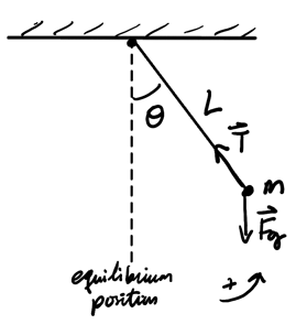
We assume there is no drag force (e.g. air resistance). By Newton's 2nd law:

\begin{align} -mgL\sin\theta &= mL^2 \frac{\text{d}^2\theta}{\text{d}t^2} \notag \\ \frac{\text{d}^2\theta}{\text{d}t^2} + \frac{g}{L}\sin\theta &= 0 \notag \end{align}

In order for this to be simple harmonic motion, we must assume that the small angle approximation can be made (that is, \(\sin\theta = \theta\)) so that it can be written in the canonical form:

\begin{align} \frac{\text{d}^2\theta}{\text{D}t^2} + \frac{g}{L}\theta = 0 \notag \end{align}

Therefore, the angular frequency is:

\begin{align} \boxed{\omega = \sqrt{\frac{g}{L}}} \end{align}

The physical pendulum, as opposed to the simple pendulum, has a mass distribution across the whole pendulum:

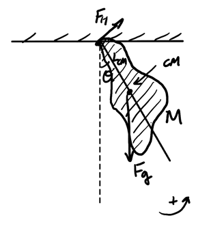
By Newton's 2nd law

\begin{align} -MgL_{\text{CM}}\sin\theta &= I\frac{\text{d}^2\theta}{\text{d}t^2} \notag \\ \frac{\text{d}^2\theta}{\text{d}t^2} + \frac{MgL_{\text{CM}}}{I}\sin\theta &= 0 \notag \end{align}

If we apply the small angle approximation, then from the canonical form we get:

\begin{align} \boxed{\omega = \sqrt{\frac{MgL_{\text{CM}}}{I}}} \end{align}

Example: Physical pendulum with rod

Consider a pendulum with a rod of mass \(M\) and length \(L\), pivoted at \(\frac{L}{4}\) from the top:

The rod has uniform mass distribution with the center of mass located \(\frac{L}{2}\) from the top. We want to determine the angular frequency \(\omega\).

The rotational inertia can be found using the parallel axis theorem:

\begin{align} I &= \frac{ML^2}{12} + M\left(\frac{L}{4}\right)^2 \notag \\ &= ML^2\left(\frac{1}{12}+\frac{1}{16}\right) \notag \\ &= \frac{7}{48}ML^2 \notag \end{align}

Now, we can find \(\omega\):

\begin{align} \omega &= \sqrt{\frac{MgL_{\text{CM}}}{I}} \notag \\ &= \sqrt{\frac{12g}{7L}} \notag \end{align}

Example: Collision with physical pendulum

Consider a physical pendulum of a rod at the equilibrium position:

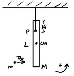
A point mass \(m\) strikes and sticks to the rod with velocity \(v_0\). We want to determine the initial angular velocity of the pendulum after the collision and the angular frequency \(\omega\).

To do this, we use conservation of angular momentum:

\begin{align} mv_0\frac{3L}{4} = I\Omega_0 \notag \end{align}

To find \(I\), we can use the parallel axis theorem to get:

\begin{align} I &= M\left(\frac{3L}{4}\right)^2 + \frac{7}{48}ML^2 \notag \\ &= \frac{9}{16}mL^2 + \frac{7}{48}ML^2 \notag \\ &= \frac{7M+27m}{48}L^2 \notag \end{align}

Plugging this back into the conservation of angular momentum, we have:

\begin{align} mv_0\frac{3L}{4} = \frac{7M+27m}{48}L^2\Omega_0 \notag \end{align}

Thus, \(\Omega_0\) is:

\begin{align} \boxed{\Omega_0 = \frac{36mv_0}{(7M+27m)L}} \notag \end{align}

We also know that:

\begin{align} \omega = \sqrt{\frac{MgL_{\text{CM}}}{I}} \notag \end{align}

However, we need to calculate a new center of mass because of the inelastic collision. To do this, we use a weighted average:

\begin{align} x_{\text{CM}} &= \frac{\left(\frac{M}{2} + m\right)L}{M+m} \notag \\ L_{\text{CM}} &= \left(x_{\text{CM}} - \frac{1}{4}\right)L \notag \\ &= \frac{M+3m}{4(M+m)}L \notag \end{align}

Plugging this back in:

\begin{align} \omega &= \sqrt{\frac{(M+m)g\frac{M+3m}{4(M+m)}L}{\frac{7M+27m}{48}L^2}} \notag \\ &= \sqrt{\frac{(M+3m)g}{4} \cdot \frac{48}{(7M+27m)L}} \notag \end{align}

Therefore, the angular frequency is:

\begin{align} \boxed{\sqrt{\frac{12g(M+3m)}{(7M+27m)L}}} \notag \end{align}

Using the canonical form, we can find the elastic potential energy and the kinetic energy of a system in SHM:

\begin{align} U_{\text{el}} &= \frac{1}{2}kx^2 = \frac{1}{2}kA^2\cos^2(\omega t + \phi) \notag \\ K &= \frac{1}{2}mv^2 = \frac{1}{2}mA^2\omega^2\sin^2(\omega t + \phi) \notag \end{align}

Then, we can add these two energies together to get the total mechanical energy of the system:

\begin{align} E = U_{\text{el}} + K &= \frac{1}{2}kA^2\cos^2(\omega t + \phi) + \frac{1}{2}mA^2\omega^2\sin^2(\omega t + \phi) \notag \\ &= \frac{1}{2}kA^2\cos^2(\omega t + \phi) + \frac{1}{2}kA^2\sin^2(\omega t + \phi) \notag \\ &= \frac{1}{2}kA^2\left[\cos^2(\omega t + \phi) + \sin^2(\omega t + \phi)\right] \notag \\ &= \frac{1}{2}kA^2 \notag \end{align}

Thus, we find that \(\boxed{E(t) = \frac{1}{2}kA^2}\), which means that we have constant mechanical energy for a system in SHM. When we plot the energy, we have the following graph:

There could also be damping: the dissipation of mechanical energy. Most of the time, damping is due to some drag force (e.g. air resistance) \(F_D = -bv\).